Visualization

This page includes some example code for visualizing and animating spin weighted spheriodal harmonics using spheroidal and matplotlib. This demo also requires ffmpeg to be installed in order to render animations and uses tqdm to generate progress bars. The Jupyter notebook that this page was compiled from is available on Github.

import matplotlib.pyplot as plt
import matplotlib.colors
from matplotlib.animation import FuncAnimation, FFMpegWriter
import numpy as np
import spheroidal
from tqdm import tqdm

We begin by constructing a unit sphere and initializing a binary colormap to represent the sign of the harmonic.

u = np.linspace(0, 2 * np.pi, 200)
v = np.linspace(0, np.pi, 100)
phi, theta = np.meshgrid(u, v)

# make sphere
x = np.sin(theta) * np.cos(phi)
y = np.sin(theta) * np.sin(phi)
z = np.cos(theta)

cmap = matplotlib.colors.ListedColormap(['tab:red', 'tab:green'])
norm = matplotlib.colors.BoundaryNorm([-1, 0, 1], ncolors=2)
ls = matplotlib.colors.LightSource(azdeg=30, altdeg=0)

Single Harmonic

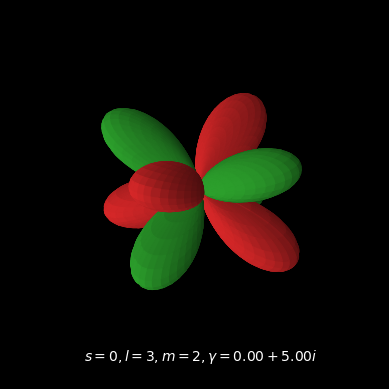
First, we will plot and animate a single harmonic. The spin weight, degree, order and spheroidicity of the harmonic can be adjusted below. Change "dark_background" to "default" to make the background white.

s, l, m, gamma = 0, 3, 2, 5j

plt.style.use('dark_background')

Plot

In this plot, the radial distance of the surface from the origin is given by the magnitude of the real component of the spin weighted spheroidal harmonic. Areas where the real component is positive are colored green and areas where it is negative are colored red.

r = np.real(spheroidal.harmonic(s,l,m,gamma)(theta,phi))
sign = np.sign(r)
r = abs(r)

fig = plt.figure()
ax = fig.add_subplot(projection='3d')
# Plot the surface
surface = ax.plot_surface(r * x, r * y, r * z, 
                          facecolors=cmap(norm(sign)), 
                          rstride=2, cstride=2,
                          lightsource=ls)

# add text with parameters and time
text = ax.text2D(
    0.2,
    0.05,
    f"$s = {s}, l = {l}, m = {m}, \gamma = {np.real(gamma):.2f} + {np.imag(gamma):.2f}i$",
    transform=ax.transAxes,
            )

# set equal aspect ratio and remove axes
ax.set_aspect("equal")
ax.axis('off')

plt.show()

Animation

Next, we will create a short animation of the harmonic rotating as the spheroidicity changes. The length of the animation in seconds and the frame rate can be set below. The function g(t) sets the spheroidicity as a function of time

length = 10
fps = 24

g = lambda t: 10*np.sin(np.pi*t/5)**2*(1 if t<5 else 1j)

When the spheroidicity is purely imaginary, the spin weighted spheroidal harmonic is prolate. When the spheroidicity is real, it is oblate. In the following animation, the harmonic rotates exactly once as the spheroidicity slowly varies from \(0\) to \(10\) and back and then from \(0\) to \(10i\) and back.

num_frames = length * fps
deg_per_frame = 360 / num_frames

# start progress bar
with tqdm(total=num_frames, ncols=80) as pbar:
    def draw_frame(i):
        # update progress bar
        pbar.update(1)

        # rotate light source
        ls.azdeg = 30-i*deg_per_frame
        # rotate camera
        ax.view_init(30, i*deg_per_frame)
        ax.set_aspect("equal")

        # recompute harmonic with updated spheroidicity
        r = np.real(spheroidal.harmonic(s,l,m,g(i/fps))(theta,phi))
        sign = np.sign(r)
        r = abs(r)

        # update plot
        global surface
        surface.remove()
        surface = ax.plot_surface(r * x, r * y, r * z, 
                                  facecolors=cmap(norm(sign)), 
                                  rstride=3, cstride=3,
                                  lightsource=ls)

        # update text
        text.set_text(f"$s = {s}, l = {l}, m = {m}, \
                      \gamma = {np.real(g(i/fps)):.2f} + {np.imag(g(i/fps)):.2f}i$")

    # save to file
    ani = FuncAnimation(fig, draw_frame, num_frames)
    FFwriter = FFMpegWriter(fps=fps)
    ani.save("single_harmonic.mp4", writer=FFwriter)
    
    # close figure so it doesn't show up in notebook
    plt.close(fig)

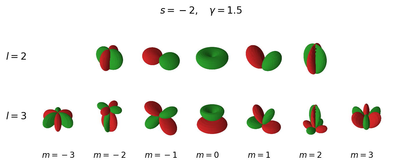
All Harmonics

Next, we will plot and animate all of the spin weight \(-2\) harmonics, starting with the \(\ell = 2\) harmonics and going up to the \(\ell = 3\) harmonics. The spheroidicity is set to \(1.5\). These parameters can be adjusted below.

s = -2
gamma = 1.5
l_min = 2
l_max = 3

plt.style.use('default')

Plot

fig, ax = plt.subplots(l_max-l_min+1, 2*l_max+1, 
                       subplot_kw=dict(projection='3d'), 
                       figsize=(8, 4), 
                       dpi=200)

l_vals = np.arange(l_min, l_max + 1)

surfaces = [] # keep track of surfaces so we can update them in the animation

for i,l in enumerate(l_vals):

    m_vals = np.arange(-l, l + 1)

    for j,m in enumerate(m_vals):
        # compute harmonic
        r = np.real(spheroidal.harmonic(s,l,m,gamma,num_terms=20)(theta,phi))
        sign = np.sign(r)
        r = abs(r)

        # plot the surface
        surfaces.append(
            ax[i,j+l_max-l].plot_surface(r * x, r * y, r * z, 
                                         facecolors=cmap(norm(sign)), 
                                         rstride=3, cstride=3,
                                         lightsource=ls)
                        )

        # add m labels to last row
        if l == l_vals[-1]:
            ax[i,j+l_max-l].text2D(
                0.2,
                -0.25,
                (f"$m = {m}$" if m >= 0 else f"$m=-{abs(m)}$"),
                transform=ax[i,j+l_max-l].transAxes,
                #size="large",
                        )
                        
# add l labels
for i,l in enumerate(l_vals):
    ax[i,0].text2D(
        -0.5,
        0.5,
        f"$l = {l}$",
        transform=ax[i,0].transAxes,
        size="large",
                )

title = ax[0,l_max].text2D(-0.5,1.4,
                           f"$s = {s},\quad \gamma = {gamma}$",
                           size="large",
                           transform=ax[0,l_max].transAxes)

# remove axes and facecolor and set equal aspect ratio for all subplots           
for axes in ax.flatten():
    axes.axis('off')
    axes.set_aspect('equal')
    axes.set_facecolor('none')

# adjust spacing between subplots
fig.subplots_adjust(wspace=0, hspace=-0.5)

Animation

Next, we will animate all of the harmonics rotating as the spheroidicity varies in the same way as in the single harmonic case above. The length, frame rate and spheroidicity can be set in the cell below.

length = 10
fps = 24

g = lambda t: 5*np.sin(np.pi*t/5)**2*(1 if t<5 else 1j)

num_frames = length * fps
deg_per_frame = 360 / num_frames

# start progress bar
with tqdm(total=num_frames, ncols=80) as pbar:
    def draw_frame(i):
        # update progress bar
        pbar.update(1)

        global title
        global ls

        # rotate light source
        ls.azdeg = 30-i*deg_per_frame
        title.set_text(f"$s = {s}, \quad \
                       \gamma = {np.real(g(i/fps)):.2f} + {np.imag(g(i/fps)):.2f}i$")

        # rotate plots
        for axes in ax.flatten():
            axes.view_init(30, i*deg_per_frame)
            axes.set_aspect("equal")

        k = 0
    
        for l in l_vals:

            m_vals = np.arange(-l, l + 1)

            for j,m in enumerate(m_vals):
                # recompute harmonic with updated spheroidicity
                r = np.real(spheroidal.harmonic(s,l,m,g(i/fps),num_terms=25)(theta,phi))
                sign = np.sign(r)
                r = abs(r)
                
                # Plot the surface
                global surfaces
                surfaces[k].remove()
                surfaces[k] = ax[l-l_min,j+l_max-l].plot_surface(r * x, r * y, r * z, 
                                                                 facecolors=cmap(norm(sign)), 
                                                                 rstride=3, cstride=3,
                                                                 lightsource=ls)
                k += 1

    # save to file
    ani = FuncAnimation(fig, draw_frame, num_frames)
    FFwriter = FFMpegWriter(fps=fps)
    ani.save("all_harmonics.mp4", writer=FFwriter)

    # close figure so it doesn't show up in notebook
    plt.close(fig)